# A tibble: 4 × 7
  term              estimate std.error statistic  p.value conf.low conf.high
  <chr>                <dbl>     <dbl>     <dbl>    <dbl>    <dbl>     <dbl>
1 (Intercept)         0.475    0.00318     149.  0          0.468     0.481
2 income             -0.0831   0.00450     -18.5 1.34e-72  -0.0920   -0.0743
3 poverty             0.0177   0.00141      12.6 2.42e-35   0.0150    0.0205
4 unemployment_rate 0.265 0.0216 12.3 7.35e-34 0.222 0.307 Model
Model
My outcome variable was continues therfore, Liner Regression Model was applied. Following is the general form of a linear regression model.
\[ Y_i = \beta_0 + \beta_1 X_{1i} + \beta_2 X_{2i} + \cdots + \beta_p X_{pi} + \varepsilon_i \]
Where: - ( Y_i ) is the dependent (response) variable, - ( X_{1i}, X_{2i}, , X_{pi} ) are the independent variables (predictors), - ( _0 ) is the intercept, - ( _1, , _p ) are regression coefficients, - ( _i (0, ^2) ) is the error term assumed to follow a normal distribution.
Probability Family Function when the outcome variable is normally distributed:
\[ Y_i \sim \mathcal{N}(\mu_i, \sigma^2), \quad \text{where} \quad \mu_i = \beta_0 + \beta_1 X_{1i} + \cdots + \beta_p X_{pi} \]
The likelihood function for all ( n ) observations is:
\[ L(\boldsymbol{\beta}, \sigma^2) = \prod_{i=1}^{n} \frac{1}{\sqrt{2\pi\sigma^2}} \exp\left( -\frac{(Y_i - \mu_i)^2}{2\sigma^2} \right) \]
3.2 Coefficients
3.3 Data Generating Mechanism
\[ \hat{\text{Gini}} = 0.475 - 0.0831 \cdot \text{Income} + 0.0177 \cdot \text{Poverty} + 0.265 \cdot \text{UnemploymentRate} \]
3.4 Model Prediction
Warning: Using `size` aesthetic for lines was deprecated in ggplot2 3.4.0.
ℹ Please use `linewidth` instead.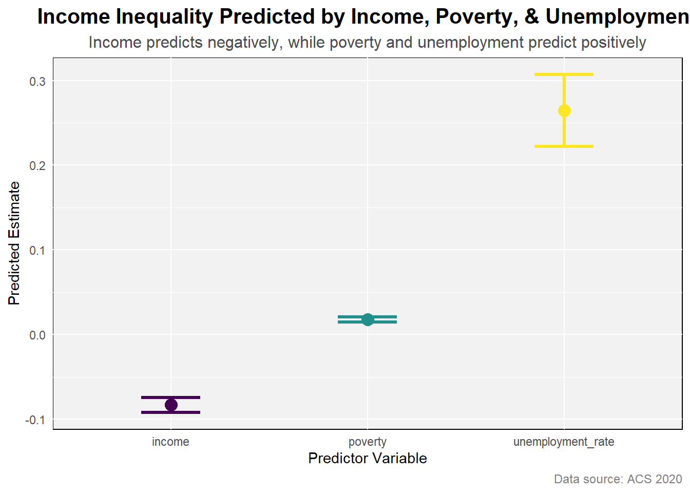
Increase in income reduces income inequality by -0.083 on the other hand, increse in poverty and unemployment rate increse income inequality by 0.018 and 0.265 respectively. Unemployment rate predicts higher than others.